Anomaly Detection using GAN's
In this post I will explain the architecture of the bigan and how can it be used for the anomaly detection problem. The papers that inspired this post are down below at the references section.
What is Anomaly Detection ?
Anomaly detection is one of the most important problems concerning multiple domains including manufacturing, Cyber-security, fraud detection and medical imaging. At its core an Anomaly Detection method should learn the data distribution of the normal samples which can be complex and high dimensional to identify the anomalous ones.
The method I will explain focuses on the reconstruction based approach to indentify the anomalous samples. By learning the data distribution and its representation, model is then able to reconstruct a sample image that is similar to the input for the inference. By defining a score function to measure the similarity between the input image and the reconstructed output, we can attain a score that can be used to identify a sample as anomalous or normal. Since the model is trained with the normal images, ideally, when the test image is normal, the reconstructed sample is expected to obtain a lower anomaly score compared to an anomalous image. That is the basis for the anomaly detection using reconstruction based approach.
Generative Adversarial Networks, or GANs are considered as a significant breakthrough in deep learning. They are used to model complex and high dimensional distributions using adversarial training. Let’s explore what that means and how we can use it for this problem.
Intuition Behind GANs
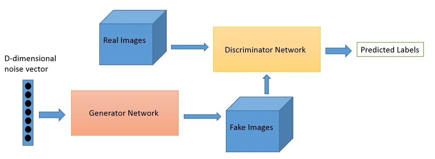
Generative Adversarial Networks consist of 2 networks, one generator and one discriminator. The generator is responsible for generating sample images that is similar to the dataset samples and tries to fool the discriminator. The purpose of the discriminator is to identify whether the image is from the dataset or it is generated by the generator, in other words to classify input images as “real” or “fake”.
The main training idea behind GANs is based on game theory and assuming that the two network are competing each other. The model is usually trained with the gradient-based approaches by taking minibatch of fake images generated by transforming random vectors sampled from \(pz(z)\) via the generator and minibatch of data samples from \(p{data}(x)\). They are used to maximize \(V(D, G)\) with respect to parameters of \(D\) by assuming a constant \(G\), and then minimizing \(V(D, G)\) with respect to parameters of \(G\) by assuming a constant \( D\).
![]()
As we can see, there are 2 loops and two terms. Let’s disect each term. They will provive useful for the BiGAN model in the next section.
Term 1

Term 2

Now there are two main loops in the equation that we need to examine. The inner loop of the discriminator and the outer loop of the Generator. If want to summarize their logic:
Inner loop is the training objective of the discriminator. It wants to maximize its probability of classifying an image as real or fake. So It needs to maximize \(D(x)\) to classify real images ( since \(D(x)\) is the probability of a discriminator identifying image as real) and it also needs to maximize \((1 - D(G(z))\) to maximize its probability for spotting fake images.
The outer loop is the training objective of the generator. Since it’s only on one of the terms we don’t need to look at the first term. Generator wants to fool the discriminator by generating more real like sample images. So in order for it to maximize its probability to get classified as real, it needs to minimize discriminator’s probability of classifying generated image as fake. So it needs to minimize \(D(G(z))\) to increase \((1 - D(G(z)))\).
Now that’s out of the way we can focus on what is BiGAN and how does it work ?
BiGAN Architecture
BiGAN is composed of a standard GAN with an additional Encoder that is simultaneously trained with the generator and discriminator. This encoder learns the mapping representation from the input image to the latent space representation (noise). This approach enables inference process much faster than the previous proposed method which is an iterative optimization process via backpropagation for each sample.
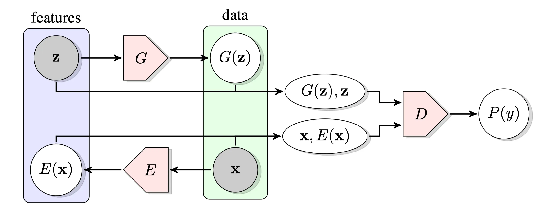
With the addition of the Encoder, the Discriminator behavior changes a little. Now the discriminator not only discriminates in data space $(z)$ or \(G(z)\)) but jointly in data and latent space tuples (\(x\), \(E(x)\)) versus (\(G(z)\) , \( z\)). Generator and encoder are trying to fool the discriminator.
Let’s explain the objective function of the BiGAN like we did with GAN.
![]()
Our objective function is similar to GAN with the difference of the noise tuple from the encoder and the latent space distribution. From the discriminator’s perspective, the pair with input image and the encoded noise of the input image should be classified as real, and the tuple with sampled noise and the generated image should be classified as fake. So again, it needs to maximize the probability of discriminating \((x, E(x))\) tuple as real and \((G(z), z)\) tuple as fake.
We can consider the encoder and generator loss in the same loop because they are both trying to fool the discriminator. Encoder wants to minimize discriminator’s probability of classifiying \((x, E(x))\). The reason for this is that in order for encoder to be an optimal one, it needs to learn the invert the input from the true data distribution, to act as \(E = G^{-1}\). Generator again wants to minimize Discriminator’s ability to spot a fake image so consequentially it wants to maximize \(D(G(z), z)\) probability.
After the training of the model is done, we can make an inference to test the model. The score function \(A(x)\) is composed of the combination of the reconstruction loss (\(L_G\)) and discrimination-based loss (\(L_D\)). The score function and its components are depicted below.

Reconstruction loss measures the difference between the input image and the reconstructed image. There are 2 types of discrimination loss that we can define. First one depends on the sigmoid cross entropy loss from the discriminator of x being a real example (class 1 in this case), and the second method for defining the discriminator loss is based on the feature matching loss with \(f_D\) returning the layer preceding the logits for the given inputs in the discriminator. This loss evaluates if the reconstructed data has similar features in the discriminator as the true sample. Samples with larger \(A(x)\) values are considered as more likely from the anomalous sample.
In this introductory post I wanted to talk about the BiGAN architecture for the anomaly detection task. In the following posts I will talk more about anomaly detection, different architectures that can be used with more detailed summary of the architectures and the training techniques.